Lab Exercise 4: Ground Control Points
Introduction:
In every UAS survey accuracy is always considered. The amount of accuracy required is always dependent on the type and application of the survey. One example where higher accuracy would be needed is a volumetric change estimation survey. Because the surveyor is comparing data collected from time one to time two at the same location, the data needs to be processed with centimeter type of accuracy. One way that UAS surveyors can improve their accuracy is through ground control points. There are many different types of ground control points that can be used to collecting data. (See below)


Figure 1. Variety of ground control points
In order to collect accurate data, GNSS (Global Navigation Satellite System) data is needed to be collected with imagery. Collecting data with no corrections using a GPS can give the surveyor 3 -5 meters horizontal accuracy, and 5 - 10 meters of vertical accuracy. However, when real time correction (RTK), SBASS, or differential GPS data is used to correct the original data a high amount of accuracy can be achieved.
- Real time correction
- Rover connects to a base station over internet connection. Rover is first taken to a benchmark and is corrected. During the survey, the RTK rover communicates with a nearby base station to which compensates for the amount of error.
- SBASS
- The United States uses WAAS for this type of correction. Ground stations transmit its highly accurate known position to geostationary satellites. Within the satellites a correction is applied and a higher amount of accuracy is transmitted to the rover.
- Differential GPS
- A base station is located at a fixed location near the survey area. This base station can be one the surveyor sets up in the field, or it can be a base station provided by the DOT. During the survey, location is being logged at the base station. Because it is a fixed point, it will achieve higher accuracy than the moving rover station. During post processing after the survey, the error is pulled from the base station and applied to the rover data.
Study Area:
Myrick Park: La Crosse, Wisconsin
43°49'22.02"N
91°13'30.62"W

Figure 2. Study area (Myrick Park, La Crosse, WI)
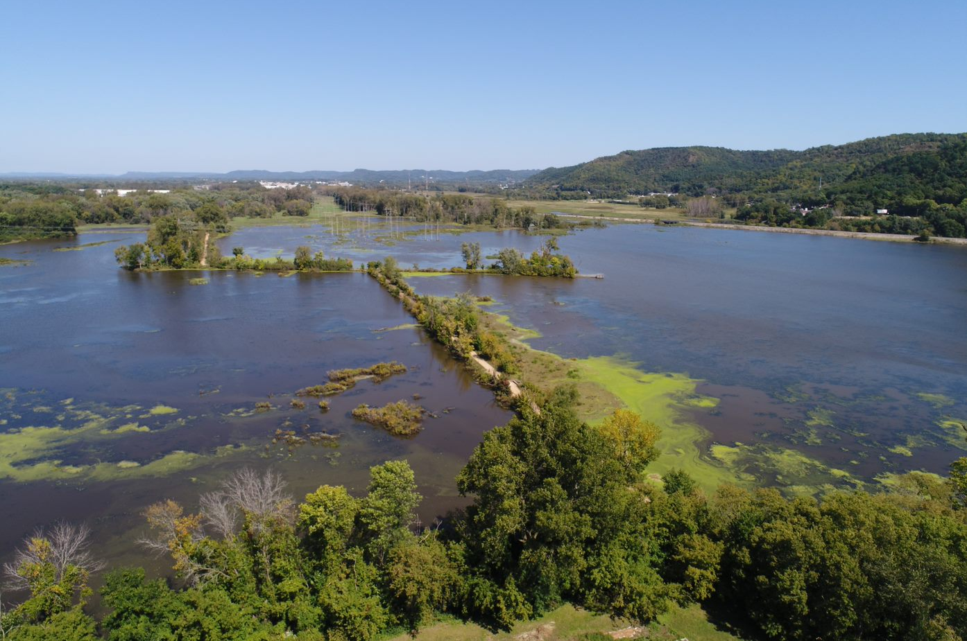
Figure 3. (below)

Figure 3 & 4. Oblique image captured by UAS of study area
Data was collected near the gun shelter located in the city of La Crosse at Myrick Park. Myrick Park was home to an old shooting range. It was not until the 1960's that Myrick Park was designated as a preserve and become submergent wetlands. When large rain events happen within the city of La Crosse, these wetlands are a 'sponge' that prevents large amounts of flooding. When the Mississippi and La Crosse River are running at high water level marks after large rain events, they are able to distribute some of their flow here so the city (which mostly sits on a flood plain) does not become overflown. Possible obstacles located within the study area are low lying powerlines, guy wires, eagles/hawks, and helicopters flying to Gunderson Hospital and low altitudes. This study area provides us with an otherwise very open area to be flow with trees reaching a maximum height of 30 - 40 feet. The land below consists of marshland/submergent wetland (70 - 80 % water, 20 - 30 % land). Water is contaminated with lead (bullets) from past land use.
Methodology:
During the survey, eight ground control points were uniformly spaced throughout the study area. GCP location was collected using uncorrected GPS rover data. The projection for logging GPS data was UTM Zone 15 N and the datum was WGS 1984. At each GCP the data was logged every second for sixty seconds.

Figure 5. GCP recording
The flight parameters of the UAS data acquisition are as listed below:

Figure 6. UAS flight parameters
Differential Correction:
- In order to achieve a higher level of accuracy at each GCP differential correction was applied using a nearby base station provided by the Wisconsin DOT.
- Base station data is logged every second of the day, 24/7. Therefore, it has a very accurately known location that can be applied to collected data by the second during post processing. The uncorrected points were loaded into GPS Pathfinder.
- From there, the Wisconsin DOT corrections were logged into the program and applied to the uncorrected points.
- After the correction, 92 % of the points were able to achieve 0 - 5 cm of accuracy (figure 7 below).

Figure 7. Accuracy of GCP points after differential correction
Results:
- Differential correction method was took less than 15 minutes (if done individually) to accomplish during post processing time.
- Accuracy of 0 - 5 cm was able to be achieve for large number of points which satisfies accuracy requirement for the survey.
- GCP installation took more time during the survey, however a greater number of accuracy was able to be achieved.
- This type of accuracy correction will not allow the surveyor to achieve sub-centimeter accuracy. It could have been improved by logging data at GCPs for longer time, however the surveyor would have only gained 1 cm of accuracy, if any.
- Using the technology we were using, accuracy can barely be improved.

Figure 8. Differential correction shift of GCP coordinates after improving accuracy (red uncorrected, yellow corrected)
Conclusion:
The expected outcome of the lab was achieved. We were able to achieve 0 - 5 cm of accuracy at our GCP locations. This lab will contribute to further study of UAS applications in volumetric change estimation at La Crescent Rock Products Inc. and NDVI comparisons over-time. Now that we have learned to achieve higher accuracy during our UAS flights, we can use UAS imagery to compare landscapes over time.