Lab 2: Image Segmentation and Nearest Neighbor Classification
By: Jackson Radenz
Introduction:
Large amounts of data and imagery are able to be collected from a desired piece of land using remote sensing techniques. The purpose for collecting data from the land is our ability to analyze and derive information from it. One of the ways of analyzing the data is the ability to classify areas in the imagery into designated land covers and land uses. This allows us to see what is happening to the land and how it is being used at a much larger scale. However, if one were to do this completely by hand this would become an incredibly time consuming task.
Object Based Image Analysis:
Luckily, programs have been developed that do this work for us using algorithms. The user is able to train the algorithm using specified parameters in order to automatically derive desired land cover classes. There are two ways to approach this. First, the user can use the pixel based approach. The algorithm goes from pixel to pixel and assigns it a class. The second way we are able to do this is through object based image analysis. The algorithm segments alike pixels and joins them together as objects. Object based image analysis provides many advantages over the pixel based approach, the largest being its ability to segment the image into objects much like humans see that enable us to make better sense of it. In this lab we explore this technique and it's advantages.

Figure 1. Object based image analysis (left) is much easier to classify, read and comprehend compared to the pixel based image analysis (right)
Objective:
- Gain a better understanding of object based image analysis segmentation techniques
- Understand parameters used in multi-spectral segmentation in eCognition
- Create a land cover map for Llyn Breing, North Wales
Methodology
- Open eCognition - 'New Project' - Open "orthol7_20423xs100999.img" imagery
- First, open the Panchromatic layer followed by the Blue, Green, Red, NIR, SWIR1, SWIR2 layers
- The image will be re-sampled to 15m
- Subset the imagery (see figure 2.)

Figure 2. Subset Selection
- Assign NIR layer to red, SWIR1 to green, and RED to blue
- Hit the icon 'Develop Rulesets 4' and create a multi-resolution segmentation process in the Process tree using a process that looks like figure 3

Figure 3. Multi-resolution segmentation process
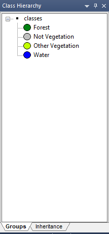
Figure 4. Class hierarchy land cover classes
- Develop a Process Tree in the form of Figure 5

Figure 5. Process Tree
- Upon doing so, you will receive a vector layer output which you will open in Arc Map, add cartographic elements, and create a land cover map
Results:
After experimenting with different segmentation input parameters the outputs below were created.
When one parameter was changed, the default parameters of the rest were as follows:


When one parameter was changed, the default parameters of the rest were as follows:
- Scale: 10
- Shape: 0.1
- Compactness: 0.5
- Layer Weighting: 1 for every layer

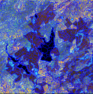
Figure 6. High Scale Factor (30)

Figure 7. Low Scale Factor (8)
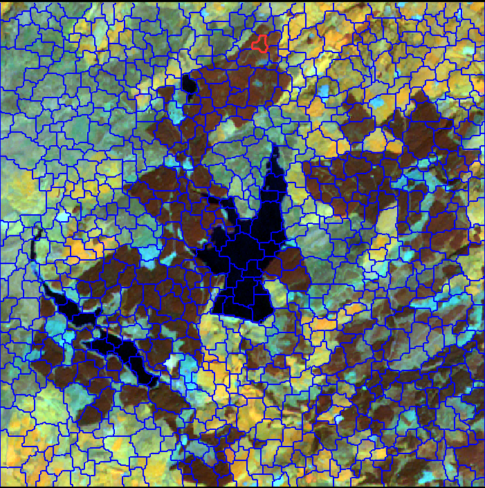
Figure 8. High Shape (0.9)

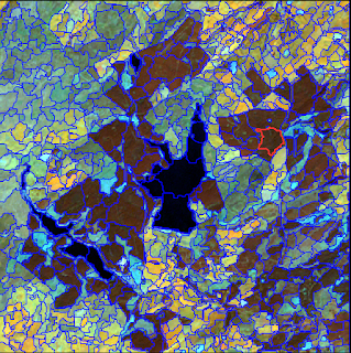
Figure 9. Low Shape (0.1)

Figure 10. High Compactness (0.9)

Figure 11. Low Compactness (0.1)

Figure 12. Panchromatic Layer (2)
Image segmentation is the cornerstone for Object Based Image Analysis. Image segmentation segments the image into homogeneous areas. For example, in Figure 9. the selected, red segment is over a very homogeneous area of forest. The program has separated this into a segment. Now that it is a segment, the mean spectral value of each layer is calculated from the group of individual pixels within the segment. Not only can the mean reflectance of each layer be calculated within a segment, many other calculations can come out of it such as, standard deviation, variation, NDVI etc. This is a great advantage for Object Based Image Analysis, because the user is then able to merge alike segments with similar spectral properties together and classify them as 'objects'. Essentially, segmentation gives a larger amount of bands to work with in the image that we can use to make sense of the image and more accurately classify the land cover.
Multi-resolution segmentation is an algorithm that segments the image using each pixel's spectral characteristics. The algorithm starts on a pixel and it moves to neighboring pixels. If the neighboring pixel values are within the threshold provided to the algorithm, the segment expands to encapsulate the pixel. The segment keeps expanding until it reaches a pixel which exceeds the threshold provided. Then, the segment is cut off and a new segment is started at that pixel. The threshold is determined by scale, shape, color, compactness, and image layer weighting. There is a trade-off between shape and color weighting. If .7 (70%) is put on shape than only .3 (30%) of the weight is put on color. The scale defines the amount of spectral variation within a segment. Therefore, if the scale is high then the image will be segmented into larger, more heterogeneous segments as compared to if the scale is low.
Figure 6. High Scale Factor (30), provided the best output for segmentation.
- Scale: 30
- Shape: 0.1
- Compactness: 0.5
- Layer weighting: Equal
The land that we were segmenting had large areas that were homogeneous. Therefore, the large scale factor was able to create these into larger segments, whereas the low scale factor (Figure 7) divided agricultural fields and forests into many segments that we would later have to merge together. Dividing the homogeneous areas of land cover is something we are trying to avoid with level 1 classification. Also, the shape weight was 0.1, which means the color weight was 0.9. Creating segments with a higher weight on the individual pixel's spectral color is a much more accurate and efficient way to segment the image.
Conclusion:

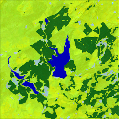
Figure 13. Nearest Neighbor Classification - mean of spectral bands (Llyn Breing, North Wales)

Figure 14. Nearest Neighbor Classification - mean of spectral bands & standard deviation (Llyn, Breing, North Wales)
Figure 15. Nearest Neighbor Classification - max pixel value NIR

Figure 16. Nearest Neighbor Classification - number of brighter objects to nearest neighbor SWIR1

Figure 17. Nearest Neighbor Classification - object's mode median values of GREEN