Lab 4

Conversion of DN to reflectance and atmospheric correction of imagery acquired by Landsat 5 Thematic Mapper

Jackson Radenz

Introduction:

Satellite acquired imagery is incredibly valuable to Geospatial Analysts in analyzing land cover change, deforestation, national defense, glacial retreat etc.  However, there must be conversions of the acquired satellite imagery before analysts are able to use the data.  The sensor in Landsat 5 Thematic Mapper collects values from each pixel in the form of digital number (DN).  These values left in digital numbers are not useful for analysis.  Therefore, Geospatial Analysts must convert the DN value of each band, in each pixel into reflectance values.  Reflectance values are values that analysts are able to use because they are able to derive spectral properties from each pixel within the data.  Not only must analysts convert DN's to reflectance, they also must correct for atmosphere scattering and transmission (figure 1.).  Because the sensor is above the atmosphere, the DN values are recorded from the top of the atmosphere.  However, we want to analyze the reflectance values that belong to the features on the surface of the earth.  Therefore, we must use ERDAS IMAGINE to convert DN's to reflectance and correct the reflectance data from atmospheric effects.         

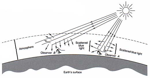
Figure 1. Atmospheric Scattering

COST Atmospheric Correction:

In order to correct for atmospheric scattering and transmission of wavelengths reflected from the surface, analyzers use the COST model which is an equation applied to each band in the imagery.  This saves a large amount of time because field data no longer needs to be collected and a very similar accuracy is achieved.  The COST model is the only model to entirely include correction for atmospheric transmittance, instead of just scattering.  Transmittance is much more costly to the image's accuracy because it is a multiplicative effect and not a additive effect.   

ERDAS IMAGINE:

ERDAS IMAGINE (figure 2.) allows the user to convert Landsat 5 Thematic Mapper bands' value from DN to Radiance using Model Maker.  After creating radiance, ERDAS allows the analyst to convert the data from radiance to top of the atmosphere reflectance and finally, atmospherically correct the reflectance values.     

Figure 2. ERDAS IMAGINE & Model Maker

Study Area & Imagery:

• Imagery Acquired from: Landsat 5 TM
• Bands Used:
• Blue
• Green 
• Red
• NIR
• SWIR 1
• SWIR 2
• Date of Imagery Acquired: 10 - 4 - 1993
• Spatial Resolution: 30 meters
• Study Area: La Crosse County, WI, USA

Methods:

• Open ERDAS IMAGINE  
• File
• Open
• Raster Layer
• Select 'lt50260291993277xxx02_subset.img' 
• Tools
• Model Maker (figure 3) 
• Input 'lt50260291993277xxx02_subset.img' into the top function
• insert (figure 4) equation into the middle function
• Save the final function as a temporary raster (figure 5)

Figure 3. Model Template

Figure 4. DN to Radiance Function

Figure 5. Temporary Raster

• Now complete previous step for Bands (2) - (6) 
• We discard Thermal Infrared Band
•  Add a function and 'STACKLAYERS' and add Bands 1-6 (figure 6)
• Add a final function and save it as 'radiance.img' (figure 6)

Figure 6. DN to Radiance Model

• Next construct a model which will go from radiance to TOA reflectance
• Your model will look like Figure 7



Figure 7. Radiance to Reflectance
• Your first function will be converting radiance to reflectance
• Figure 8
• Do the same for each band

Figure 8. Radiance to Reflectance

• Save the output as a temporary layer just as you did above, and the next function will be an 'either or' statement'
• In an essence, this statement is saying keep the reflectance value if it is positive, if it is negative give it a zero
• We give it a zero because we are not concerned with negative reflectance values (Figure 9)

Figure 9. 'Either Or' Statement

• Save each output as a temporary layer and stack them (same as above)
• Top of atmosphere reflectance is now calculated
• Finally, surface reflectance must be calculated
• The COST model will be used in this lab for atmospheric correcting
• Open the Excel spreadsheet and change the values in each band according to the metadata and tables provided
• Now, in 'model builder' load the TOA reflectance model
• The only function that will be changed is the first function
• Insert the equation from your excel spread sheet (Figure 10)

Figure 10. Atmospheric Correction

• Do the same for bands 1-6 
• Surface reflectance is now calculated
• Finally, calculate NDVI
• The NDVI model will look like (Figure 11)
• DN, surface reflectance, and top of the atmosphere reflectance will be your inputs, respectively

Figure 11. NDVI

• Look at Figure 12 for the function equation

Figure 12. NDVI calcuation

• Press the lighting bolt to run it and NDVI is calculated.  Repeat for each desired output (DN, top of the atmosphere reflectance, etc.)

Discussion:

I opened each NDVI output in ERDAS Imagine and compared each output value in 10 pixels.  From there, I created a data table recording NDVI values for each output at the same pixels (Figure 13).

    Figure 13. NDVI value chart

The images below are the NDVI outputs from DN, top of atmosphere reflectance, and surface reflectance.  

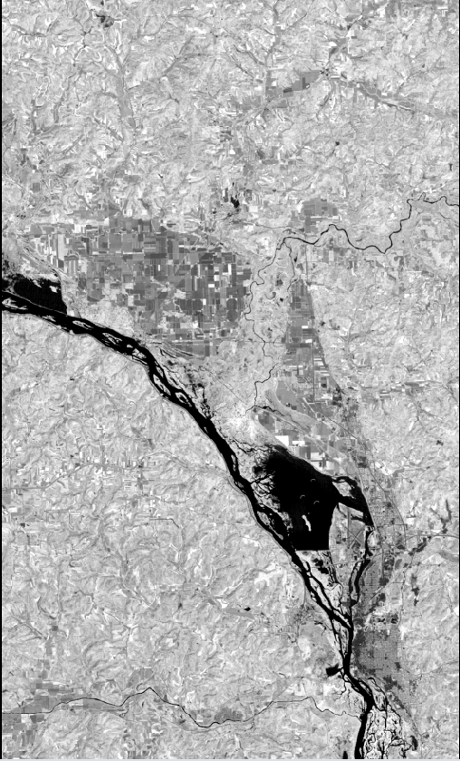
Figure 14. DN NDVI

Figure 15. TOA Reflectance NDV

Figure 16. Surface Reflectance NDVI

Conclusion:

Upon examining the NDVI values of the DN output, TOA reflectance output, and the surface reflectance output for individual pixels, I found that the further the processing, the more accurate NDVI output. First, the DN NDVI output values were of little significance. Pixel 4 had an NDVI value of 0.161, however TOA and surface reflectance both had negative NDVI values. The DN NDVI values did not correlate positively or negatively with the surface and TOA reflectance values and therefore should be deemed inconsistent. Also, the DN values were always positive, whereas both the NDVI TOA reflectance and surface reflectance values were occasionally negative. The NDVI values were always higher for the surface reflectance output. Also, I found that the NDVI values for surface reflectance flux-gated less than the values of TOA reflectance for each pixel in a given land cover class. Simply, surface reflectance NDVI values had much more consistent values. The values for surface reflectance NDVI were always larger than TOA reflectance. This is accurate because the surface reflectance corrects for atmospheric scattering and transmission, while the TOA reflectance does not. Atmospheric scattering will lower reflectance values because the wavelengths reflected from the features on the earth are scattered back down to the earth, within the atmosphere, or back out to space instead of the sensor on Landsat 5 TM.