Lab 6
MODIS TO MONITOR NDVI CHANGES
By: Jackson Radenz
Introduction:
Remote sensing gives us the ability to monitor vegetation growing seasons and the browning or greening of vegetation over large sums of area using imagery collected by MODIS. MODIS's imagery is able to capture large areas in a very fast amount of time. In other words, MODIS has a very low spatial resolution, but high temporal resolution, which allows geographers to efficiently analyze vegetation patterns over a large temporal domain. The ability to study vegetation growing cycles and its browning or greening is becoming increasingly more important in helping us understand climate change and it's effect on vegetation. During this exercise I will analyze Minnesota and Wisconsin's browning or greening using MODIS acquired imagery.
MODIS:
MODIS is aboard both Terra (collects imagery over land) and Aqua (collects imagery over water). Aboard Terra, MODIS is able to pass north to south across the equator in the morning. This allows to take imagery of land over sunlit parts of the earth. MODIS is able to acquire imagery over the entire surface of the earth every 1 - 2 days. MODIS hyper spectral sensor which consists of 36 bands allows analysts to further understand earth's climate and changes occurring on land.

Figure 1. Imagery collected by MODIS
Data:
- Imagery collected by: MODIS
- Date Collected: 2000 - 2017
- Type: 16 - day composite from 2000 - 2017
- Zone: h11v4 - Upper Midwest, Great Lake Region
Methodology:
- Download data from https://urs.earthdata.nasa.gov/
- Move the downloaded data to your working folder
- Open ENVI
- First we must combine the composites to make annual mean NDVI layers.
- Open Band Math
- type 'float((b1+b2+b3+b4+b5)/5)'
- Assign each composite layer to b1 - b5. A mean annual NDVI layer will be produced.
- Stack each downloaded composite image
- To do go into:
- Basic Tools
- Layer Stacking
- Stack each layer into the Layer Stacking Parameters window (Figure 2.)

- Figure 2. Layer Stacking Parameters window
- We must apply a mask to each layer so that we are positive the data we are working with is land. Therefore, we want to scrap any negative NDVI values.
- Open Basic Tools
- Open Masking - Build Mask
- Load each layer (2000 - 2017) into the window
- Build a mask that will result in giving all areas that were ever negative throughout all the bands a 0 and all the areas that were never negative a 1
- Save File
- Open Basic Tools
- Open Masking - Apply Mask
- Apply the mask to the stacked imagery. This will create an output of each layer with positive NDVI values being unchanged and negative NDVI values becoming 0.
- In order to get our stacked layer to work in TerrSet we must apply a scale factor of (0.0001) to the data.
- Open Basic Tools
- Open Band Math
- Write the equation 'b1*10000' to make it a unsigned 16 bit
- Assign your stacked NDVI image to b1 (Figure 3)
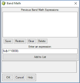
- Figure 3. Band Math
- Now we must produce a z-profile (Figure 4)

- Figure 4. Z-Profile
- Go to tools
- Open z-profile
- load 2000, 2005, 2015 bands and take z-profiles of each
- Repeat steps 8-11, but scale back down the data set so that it is between 0-1


Results:
Using pixel locator I was able to create z-profiles for the location of 43.806262N , -91.201492E. The red line on the z-profile is the band. Therefore, in this case it is representing the year in the stacked layer. The signed integer z-profiles for the location for 2000, 2005, and 2015 is as follows.


Figure 5. Z-profile for 2000

Figure 6. Z-profile for 2005

Figure 7. Z-profile for 2015
Discussion:
The z-profile allows us to visually analyze which years the vegetation has browned and which years the vegetation and greened. The z-profile allows us to see that in 2006 and 2012 the pixel located in La Crosse county experienced browning.
There are a few limitations with the NDVI band ratio. One limitation of the NDVI band ratio is that is does not account for areas of vary sparse vegetation. Therefore, the bare soil in areas of vary sparse vegetation can throw off NDVI in that area and make it become inaccurate. Another limitation of NDVI is that it areas in high biomass need improved sensitivity to NDVI. In areas of high biomass, NDVI could be measuring the values from the same tree twice. Therefore, NDVI values in areas with very dense vegetation will be thrown off or inaccurate. Here EVI index would be deem appropriate.
Conclusion:
Analyzing NDVI over time in large areas allow us to make connections between human/climate processes and its impact on vegetation. For example, if we see a browning trend near Milwaukee, we can predict that perhaps there has been urban sprawl. Coupled with the right data, we are able to make connections on exactly what our human processes is doing to vegetation. Or, if we saw a browning trend for most of the pixels in 2006 across Wisconsin we could look at climate data and realize that perhaps a drought affected the vegetation's NDVI for that year. This high temporal MODIS imagery, coupled with ENVI's ability to stack and average layers, allow us to make connections between vegetation and other processes that we would've otherwise been unable to make.